
VBA Script - Automated Reporting
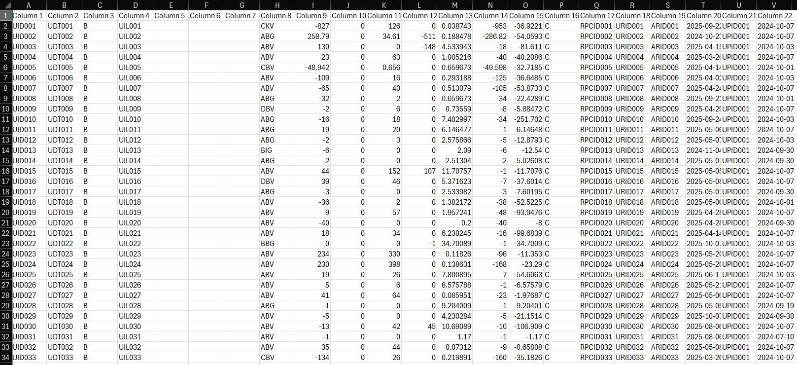
Before Script Run
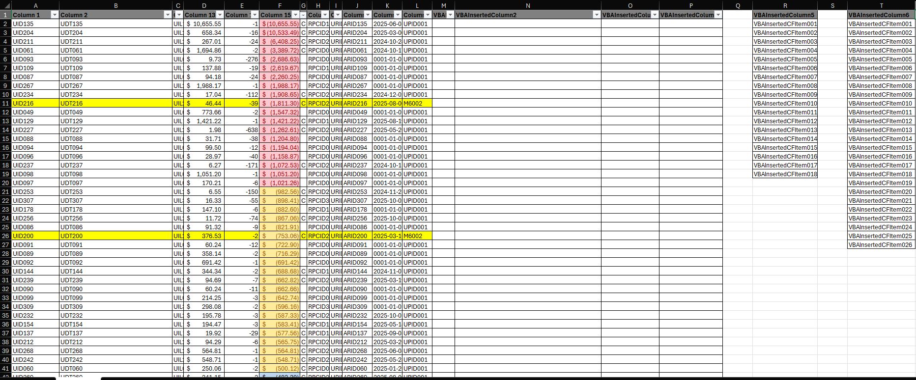
After Script Run
Overview | Description
Automated Data Processing & Formatting
Column Management: Removes unnecessary columns and restructures data for clarity.
Data Reorganization: Copies and inserts key columns to ensure consistency.
Sorting & Filtering: Sorts data in descending order and applies filters for easy navigation.
Data Categorization: Adds fields for responsibility, location, and issue classification.
Drop-Down Lists: Implements data validation for standardized selections.
Conditional Highlighting:
- Flags critical values exceeding thresholds.
- Marks outdated records based on date criteria.
Formatting Enhancements: Applies borders to key cells and ensures uniform styling.
Summary Calculations:
- Inserts formulas to count entries and sum key figures.
- Formats financial data in accounting style.
Column Resizing & Alignment: Adjusts widths for readability and aligns headers properly.
See full script below. ____________________________________________________________________________________________________________________
                            Sub DataProcessingScript()
                            Dim ws As Worksheet
                            Set ws = ActiveSheet
                            Dim row As Long, lastRow As Long

                            ' Step 1: Remove unnecessary columns to ensure correct data structure
                            ws.Columns("V").Delete
                            ws.Columns("L").Delete
                            ws.Columns("K").Delete
                            ws.Columns("J").Delete
                            ws.Columns("I").Delete
                            ws.Columns("H").Delete
                            ws.Columns("G").Delete
                            ws.Columns("F").Delete
                            ws.Columns("E").Delete
                            ws.Columns("C").Delete

                            ' Step 2: Add new column headers in row 1 starting from column M
                            ws.Cells(1, 13).Value = "Category 1"
                            ws.Cells(1, 14).Value = "Notes"
                            ws.Cells(1, 15).Value = "Issue Type"
                            ws.Cells(1, 16).Value = "Department"
                            ws.Cells(1, 18).Value = "Issue List"
                            ws.Cells(1, 20).Value = "Responsible Party"

                            ' Step 3: Format headers (gray fill and bold text)
                            With ws.Range("A1:P1,R1,T1")
                                .Interior.Color = RGB(128, 128, 128)
                                .Font.Bold = True
                            End With

                            ' Step 4: Remove rows based on specific criteria (Column L starts with "K")
                            For row = ws.Cells(ws.Rows.Count, "L").End(xlUp).row To 2 Step -1
                                If Left(ws.Cells(row, "L").Value, 1) = "K" Then
                                    ws.Rows(row).Delete
                                End If
                            Next row

                            ' Step 5: Remove rows that contain "CC" in Column C
                            For row = ws.Cells(ws.Rows.Count, 3).End(xlUp).row To 2 Step -1
                                If ws.Cells(row, 3).Value = "CC" Then
                                    ws.Rows(row).Delete
                                End If
                            Next row

                            ' Step 6: Apply conditional formatting to Column F based on value thresholds
                            With ws.Range("F2:F" & ws.Cells(ws.Rows.Count, "F").End(xlUp).row)
                                .FormatConditions.Add Type:=xlCellValue, Operator:=xlLess, Formula1:="=-1000"
                                .FormatConditions(1).Interior.Color = RGB(255, 199, 206)
                                .FormatConditions(1).Font.Color = RGB(156, 0, 6)

                                .FormatConditions.Add Type:=xlCellValue, Operator:=xlLess, Formula1:="=-500"
                                .FormatConditions(2).Interior.Color = RGB(255, 235, 156)
                                .FormatConditions(2).Font.Color = RGB(156, 87, 0)

                                .FormatConditions.Add Type:=xlCellValue, Operator:=xlLess, Formula1:="=-100"
                                .FormatConditions(3).Interior.Color = RGB(189, 215, 238)
                                .FormatConditions(3).Font.Color = RGB(0, 0, 0)

                                .FormatConditions.Add Type:=xlCellValue, Operator:=xlLess, Formula1:="=-50"
                                .FormatConditions(4).Interior.Color = RGB(244, 176, 132)
                                .FormatConditions(4).Font.Color = RGB(0, 0, 0)

                                .FormatConditions.Add Type:=xlCellValue, Operator:=xlGreaterEqual, Formula1:="=-50"
                                .FormatConditions(5).Interior.Color = RGB(201, 201, 201)
                                .FormatConditions(5).Font.Color = RGB(0, 0, 0)
                            End With

                            ' Step 7: Sort Column F (Numeric Values) from smallest to largest
                            lastRow = ws.Cells(ws.Rows.Count, 1).End(xlUp).row
                            ws.Sort.SortFields.Clear
                            ws.Sort.SortFields.Add Key:=ws.Range("F1:F" & lastRow), Order:=xlAscending
                            With ws.Sort
                                .SetRange ws.Range("A1:P" & lastRow)
                                .Header = xlYes
                                .MatchCase = False
                                .Orientation = xlTopToBottom
                                .Apply
                            End With

                            ' Step 8: Populate reference lists for Issue Types and Responsible Parties
                            Dim issueTypes As Variant
                            issueTypes = Array("Type A", "Type B", "Type C", "Type D", "Type E", _
                                            "Type F", "Type G", "Type H", "Type I", "Type J", _
                                            "Type K", "Type L", "Type M", "Type N", "Type O")

                            Dim i As Integer
                            For i = 0 To UBound(issueTypes)
                                ws.Cells(i + 2, 18).Value = issueTypes(i)
                            Next i

                            Dim responsibleParties As Variant
                            responsibleParties = Array("Team 1", "Team 2", "Team 3", "Team 4", "Team 5", _
                                                    "Team 6", "Team 7", "Team 8", "Team 9", "Team 10")

                            Dim j As Integer
                            For j = 0 To UBound(responsibleParties)
                                ws.Cells(j + 2, 20).Value = responsibleParties(j)
                            Next j

                            ' Step 9: Highlight rows in Column L if value starts with "M6"
                            For Each cell In ws.Range("L2:L" & lastRow)
                                If Left(cell.Value, 2) = "M6" Then
                                    ws.Range("A" & cell.row & ":L" & cell.row).Interior.Color = RGB(255, 255, 0)
                                End If
                            Next cell

                            ' Step 10: Add drop-down lists for Issue Types and Responsible Parties
                            With ws.Range("O2:O" & lastRow).Validation
                                .Delete
                                .Add Type:=xlValidateList, AlertStyle:=xlValidAlertStop, Operator:= _
                                    xlBetween, Formula1:="=$R$2:$R$" & UBound(issueTypes) + 2
                                .IgnoreBlank = True
                                .InCellDropdown = True
                            End With

                            With ws.Range("P2:P" & lastRow).Validation
                                .Delete
                                .Add Type:=xlValidateList, AlertStyle:=xlValidAlertStop, Operator:= _
                                    xlBetween, Formula1:="=$T$2:$T$" & UBound(responsibleParties) + 2
                                .IgnoreBlank = True
                                .InCellDropdown = True
                            End With

                            ' Step 11: Apply borders to key data columns
                            ws.Range("A1:P" & lastRow).Borders.LineStyle = xlContinuous

                            ' Step 12: Insert formulas for summary statistics
                            ws.Cells(lastRow + 2, 1).Formula = "=COUNTA(A2:A" & lastRow & ")"
                            ws.Cells(lastRow + 2, 5).Formula = "=SUMPRODUCT(ABS(E2:E" & lastRow & "))"
                            ws.Cells(lastRow + 2, 6).Formula = "=SUMPRODUCT(ABS(F2:F" & lastRow & "))"

                            ' Step 13: Format summary statistics
                            ws.Cells(lastRow + 2, 5).Style = "Comma"
                            ws.Cells(lastRow + 2, 6).Style = "Currency"
                            ws.Cells(lastRow + 2, 6).NumberFormat = "$#,##0.00"

                            ' Step 14: Format numeric columns with accounting style
                            With ws.Range("F2:F" & lastRow)
                                .NumberFormat = "_($* #,##0.00_);_($* (#,##0.00);_($* '-'??_);_(@_)"
                            End With

                            ' Step 15: Adjust column widths for readability
                            ws.Columns.AutoFit

                            ' Step 16: Apply filters to headers
                            ws.Range("A1:P1").AutoFilter

                            ' Step 17: Finalize by selecting cell A1
                            ws.Cells(1, 1).Select
                        End Sub