
VBA Script - Automated Reporting
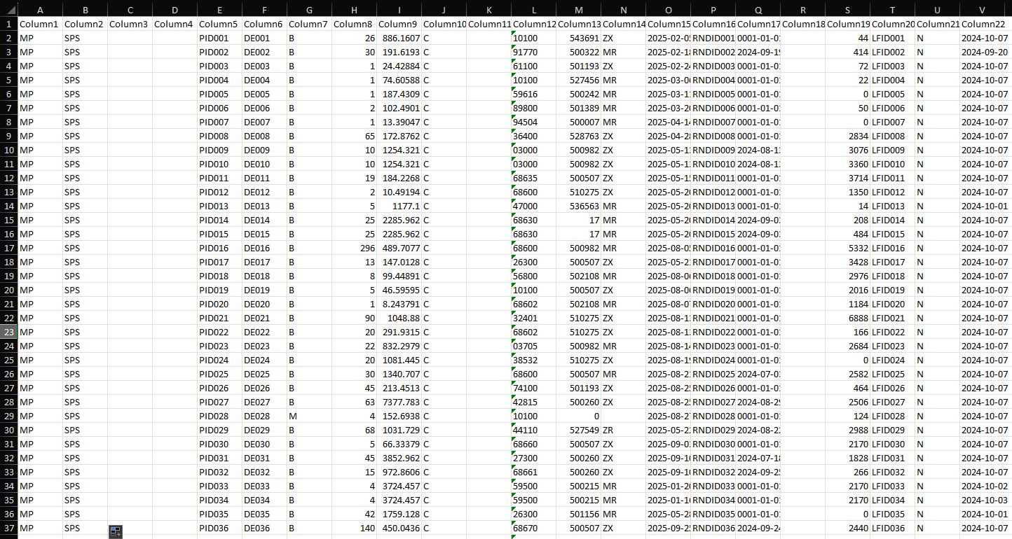
Before Script Run
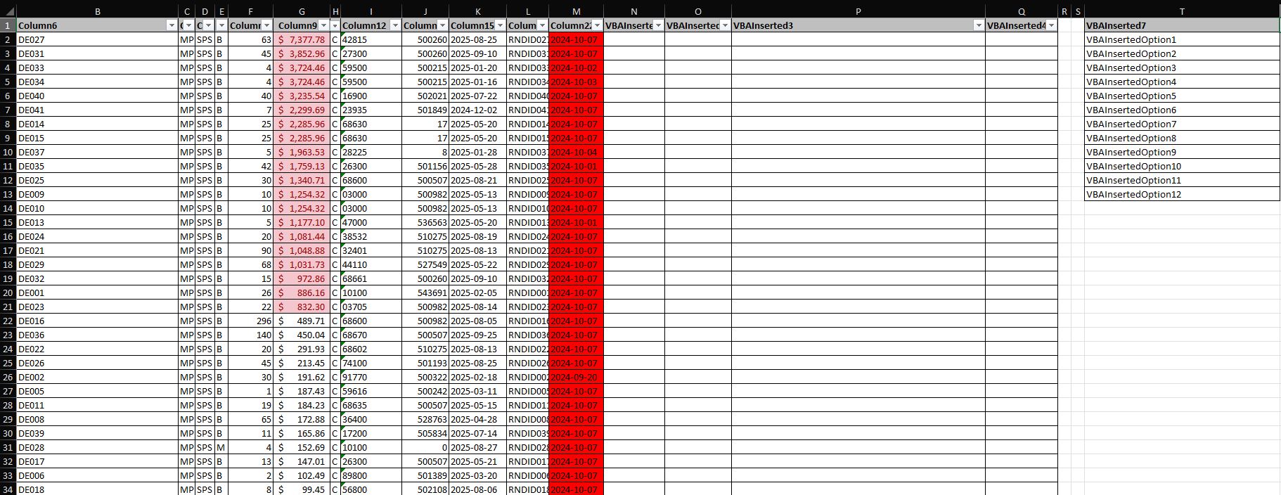
After Script Run
Overview | Description
Automated Data Structuring & Cleanup
Column Optimization: Removes unnecessary columns and restructures the dataset by copying and repositioning key fields for improved clarity.
Sorting & Filtering: Sorts numerical values in descending order and applies filters to streamline data analysis.
Data Categorization: Adds new fields to capture details such as responsible parties, locations, and classification codes for better tracking.
Drop-Down Selection: Implements a predefined list of selectable values, ensuring standardized data entry for key columns.
Conditional Formatting:
- Highlights numerical values that exceed a certain threshold to flag important records.
- Identifies outdated entries by marking dates older than a specified timeframe.
Border & Layout Enhancements: Applies borders selectively to key columns while maintaining a clean, structured format.
Summary Calculations:
- Inserts automated formulas to count entries and sum relevant numerical values.
- Ensures financial figures are formatted properly for easy interpretation.
Column Adjustments & Alignment: Resizes columns for optimal readability and aligns headers for a polished final layout.
____________________________________________________________________________________________________________________
    Sub AutomatedReportScript()
    Dim ws As Worksheet
    Set ws = ActiveSheet
    Dim lastRow As Long
    Dim lastRowT As Long
    Dim colWidths As Object
    Dim cell As Range
    Dim validationRange As Range
    Dim dataValidationCell As Range
    Dim firstRowCell As Range
    Dim dateValue As Date

    ' Step 1: Remove the specified columns C, D, K, N, Q, R, S, T, U
    ws.Columns("U").delete
    ws.Columns("T").delete
    ws.Columns("S").delete
    ws.Columns("R").delete
    ws.Columns("Q").delete
    ws.Columns("N").delete
    ws.Columns("K").delete
    ws.Columns("D").delete
    ws.Columns("C").delete

    ' Step 2: Copy columns C and D and insert them before columns A and B
    ws.Columns("C:D").Copy  ' Copy columns C and D
    ws.Columns("A:B").Insert Shift:=xlToRight  ' Insert copied cells before columns A and B

    ' Delete the original columns C and D
    ws.Columns("E:F").delete  ' The original C and D are now shifted to columns E and F

    ' Step 3: Add new columns in positions N, O, P, and Q
    ws.Cells(1, 14).Value = "Responsible"      ' Column N
    ws.Cells(1, 15).Value = "Aisle Found"      ' Column O
    ws.Cells(1, 16).Value = "Comments"         ' Column P
    ws.Cells(1, 17).Value = "Reason Codes"     ' Column Q

    ' Step 4: Sort Column G from greatest to least
    lastRow = ws.Cells(ws.Rows.Count, "A").End(xlUp).row
    ws.Sort.SortFields.Clear
    ws.Sort.SortFields.Add Key:=ws.Range("G1:G" & lastRow), Order:=xlDescending
    With ws.Sort
        .SetRange ws.Range("A1:Q" & lastRow)
        .Header = xlYes
        .Apply
    End With

    ' Step 5: Insert a new column in T named "Reason Codes" with the specified list
    ws.Columns("T").Insert
    ws.Cells(1, 20).Value = "Reason Codes"  ' Column T
    Dim reasonCodes As Variant
    reasonCodes = Array("Found in CC 999 Location", "Found in GS", "Found in PW", "Found in QA", _
                        "Found in QL Main Bldg", "Found in QL MHC", "Found in QL Outside", _
                        "Found in QL TES", "Found in QL Trailers", "Moved to CC for further Review or Approval", _
                        "Wrote Off- Could Not Locate", "Wrote Off- Did Not Review")
    Dim i As Integer
    For i = 0 To UBound(reasonCodes)
        ws.Cells(i + 2, 20).Value = reasonCodes(i)
    Next i

    ' Step 6: Apply cell borders to A through Q, excluding R and S
    For Each cell In ws.Range("A1:Q" & lastRow)
        If Not cell.Column = 18 And Not cell.Column = 19 Then  ' Skip Columns R and S
            cell.Borders.LineStyle = xlContinuous
        End If
    Next cell

    ' Step 7: Ensure all cells in column T with data have borders
    lastRowT = ws.Cells(ws.Rows.Count, "T").End(xlUp).row ' Find the last used row in column T
    For Each cell In ws.Range("T1:T" & lastRowT)
        If cell.Value <> "" Then ' Apply borders only to cells with data
            cell.Borders.LineStyle = xlContinuous
        End If
    Next cell

    ' Step 8: Add Data Validation Drop Down in Column Q
    Set validationRange = ws.Range("T2:T13") ' Define the range for dropdown list values
    For Each dataValidationCell In ws.Range("Q2:Q" & lastRow)
        With dataValidationCell.Validation
            .delete ' Clear any existing validation
            .Add Type:=xlValidateList, AlertStyle:=xlValidAlertStop, Operator:=xlBetween, Formula1:="=" & validationRange.Address
            .IgnoreBlank = True
            .InCellDropdown = True
            .ShowInput = True
            .ShowError = True
        End With
    Next dataValidationCell

    ' Step 9: Conditional format Column G for cells > 500
    With ws.Range("G2:G" & lastRow).FormatConditions.Add(Type:=xlCellValue, Operator:=xlGreater, Formula1:="500")
        .Interior.Color = RGB(244, 199, 206)
        .Font.Color = RGB(156, 0, 6)
    End With

    ' Step 10: Conditional format Column M for dates more than 71 hours older than today
    For Each cell In ws.Range("M2:M" & lastRow)
        If cell.Value <> "" And IsDate(cell.Value) Then
            dateValue = cell.Value
            If dateValue < (Now() - (71 / 24)) Then
                cell.Interior.Color = RGB(255, 0, 0)
                cell.Font.Color = RGB(0, 0, 0)
            End If
        End If
    Next cell

    ' Step 11: Apply background color and text formatting to A through Q and T headers
    For Each firstRowCell In ws.Range("A1:Q1")
        If firstRowCell.Column <> 18 And firstRowCell.Column <> 19 Then
            firstRowCell.Interior.Color = RGB(191, 191, 191)
            firstRowCell.Font.Color = RGB(0, 0, 0)
            firstRowCell.Font.Bold = True
        End If
    Next firstRowCell
    ws.Range("T1").Interior.Color = RGB(191, 191, 191)
    ws.Range("T1").Font.Color = RGB(0, 0, 0)
    ws.Range("T1").Font.Bold = True

    ' Step 12: Add filters to A through Q headers
    ws.Range("A1:Q1").AutoFilter

    ' Step 13: Resize columns and center-align header in P1
    Set colWidths = CreateObject("Scripting.Dictionary")
    colWidths.Add "A", 12.86
    colWidths.Add "B", 32.14
    colWidths.Add "C", 2.71
    colWidths.Add "D", 3.29
    colWidths.Add "E", 2#
    colWidths.Add "F", 8.43
    colWidths.Add "G", 8.43
    colWidths.Add "H", 1.43
    colWidths.Add "I", 11.71
    colWidths.Add "J", 8.86
    colWidths.Add "K", 11#
    colWidths.Add "L", 7.86
    colWidths.Add "M", 10.43
    colWidths.Add "N", 11.71
    colWidths.Add "O", 12.86
    colWidths.Add "P", 50.86
    colWidths.Add "Q", 14#
    colWidths.Add "R", 2#
    colWidths.Add "S", 2#
    colWidths.Add "T", 39#

    ' Apply column widths
    Dim colLetter As Variant
    For Each colLetter In colWidths.Keys
        ws.Columns(colLetter).ColumnWidth = colWidths(colLetter)
    Next colLetter

    ' Center-align P1 (header for column P)
    With ws.Range("P1")
        .HorizontalAlignment = xlCenter
        .VerticalAlignment = xlCenter
    End With

    ' Step 14: Format column G to Accounting format
    With ws.Columns("G")
        .NumberFormat = "_($* #,##0.00_);_($* (#,##0.00);_($* '-'??_);_(@_)"
    End With

    ' Step 15: Insert formulas at the bottom of columns A, F, and G
    Dim lastRowA As Long, lastRowF As Long, lastRowG As Long
    lastRowA = ws.Cells(ws.Rows.Count, "A").End(xlUp).row
    lastRowF = ws.Cells(ws.Rows.Count, "F").End(xlUp).row
    lastRowG = ws.Cells(ws.Rows.Count, "G").End(xlUp).row
    ws.Cells(lastRowA + 2, 1).Formula = "=COUNTA(A1:A" & lastRowA & ")"
    ws.Cells(lastRowF + 2, 6).Formula = "=SUM(F1:F" & lastRowF & ")"
    ws.Cells(lastRowG + 2, 7).Formula = "=SUM(G1:G" & lastRowG & ")"
    With ws.Cells(lastRowG + 2, 7)
        .NumberFormat = "_($* #,##0.00_);_($* (#,##0.00);_($* '-'??_);_(@_)"
    End With
End Sub